y25 - Graphs in 2.5 dimensions
Werner Jainek
I. Introduction
1. The purpose of graph visualization
A graph can capture relationships between a collection of entities. The entities are modeled as nodes of the graph, the relationships as directed or undirected edges of the graph. In formal notation, a graph G is defined as G = (N,E), where N is the set of nodes and E is the set of edges.
In this purely abstract form, a graph can capture all kinds of complex relationships between entities, but it is difficult for humans to access this information. The main purpose of graph visualization is to display the information present in a graph in way that is easily understandable for humans.
Exactly defining what is "easily understandable" by humans is not a simple matter though, which is why many of the useful visualization mechanisms existent today have evolved from a trial-and-error approach.
However, there are some properties of the human visual system that may be relevant for graph visualization: it is able to detect symmetries even in complex scenarios, it is easily able to group entities together based on their distance, color or shape, etc. A good visualization algorithm probably makes use of at least some of these properties to convey the information stored in a graph to the viewer.
2. Existing visualization methods
2D layouts
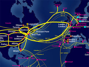
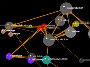
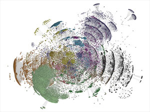
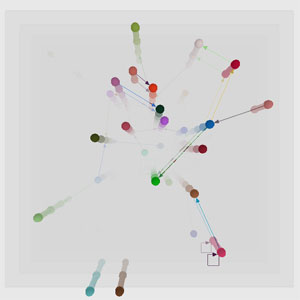
There exist a myriad of algorithms designed to lay out graphs in a two dimensional space. Below are results of some impressive existing layout algorithms:
In these examples, the position of nodes and edges in two-dimensional space play a very important role in conveying information to the viewer - together with their color and shape.
3D layouts
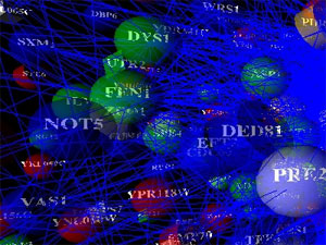
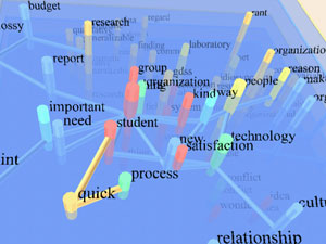
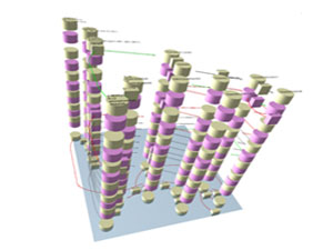
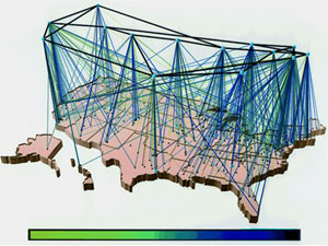
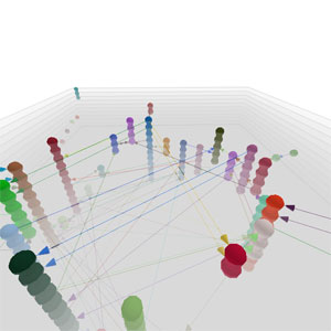
More recently, attempts have been made to convey information through the position of nodes and edges in three-dimensional space. Below are some examples of that endeavor:
In my view, the above examples all suffer from one mayor problem: it is difficult for humans to reconstruct the three-dimensional information of a scene when looking at a two-dimensional projection thereof. This is especially true for abstract three-dimensional objects such as graphs.
The main reason for this "hardness" is that the 2D projection is ambiguous: one point on the 2D image corresponds to a line, i.e. infinitely many points in 3D space.
Research in the field of Computer Vision aims to enable computers to solve this ambiguity and to perform the reconstruction process.
This in turn seems only possible by using previous information about the scene at hand when doing the reconstruction. When dealing with projections of the real world (e.g photographs), the human visual system shows its remarkable capability of inferring the 3D structure from the 2D projection. It is presumably using many assumptions and constraints that the real world imposes on the projection:
- Objects are generally composed of surfaces that don't have fast changing gradients, i.e. they are pretty smooth.
- Each object adheres to several "composition rules", e.g. a human face is pretty much oval, has ears to the left and right, a nose in the middle, etc. A tree starts with a stem, has branches and finally leafs. When some of these features are detected (e.g. one ear, the side of a nose, half a mouth), the three-dimensional configuration can be predicted from the "composition rules".
- The relationships of objects to one another is not arbitrary, e.g. a house can't stand on the head of a person. If it would, we probably could still infer the 3D information of each object individually (the house, the person), but combining these in a coherent 3D scene would be very hard.
So while these constraints help us to disambiguate real world scenes, when looking at the projection of an abstract object such as a graph, they don't help us a bit, since they don't hold anymore. All of a sudden, the remarkable achievement of the visual system breaks down and reconstruction becomes a very hard process for us as well.
While realizing the problems mentioned above can be a setback at first, it can also help in designing good three-dimensional layout algorithms. One would hope that by using several constraints when positioning nodes and edges of a graph in three-dimensional space, humans will be better able to comprehend the 3D structure of the displayed graph.
Indeed, the picture below shows a very promising approach in laying out a graph that is a tree in graph-theoretical sense:
Edges are modeled as branches and nodes as leafs. By borrowing the constraints of a real world tree (branches have to grow upwards most of the time, branches become thinner, shorter and more numerous as we move up the tree), this layout algorithm produces 3D structures that can be easily inferred from a 2D projection by human viewers.
2.5D layouts
Motivated by the success of using real world constraints when laying out a graph in three dimensions, we could search for another set of constraints that also lead to "more understandable" three-dimensional structures of graphs.
One such set of constraints results in structures that are said to have two and a half dimensions. They are:
- A graph is composed of multiple layers.
- Each layer lives on a 2D plane inside the 3D space. All layer planes are parallel and have a specific distance to each other.
- Nodes can only be positioned inside a layer.
- Edges are entirely inside one layer, connecting two nodes from that layer. (A relaxation of this constraints is to also allow layer edges that connect nodes possibly lying in different layers.)
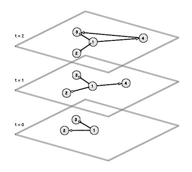
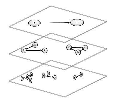
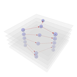
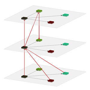
This set of constraints restricts the use of the third dimension drastically (hence the name 2.5D): only layers have the full freedom of three-dimensional coordinates. Once they are set, all nodes and edges inside the layer cannot "break out" of the 2D plane determined by the layer. Below is a schematic drawing of such a 2.5D layout:
The hope is that 2.5D layouts of graphs can still be easily grasped by humans, even though the set of constraints is somewhat more abstract (but therefore more general) than the set of constraints in the tree-example. Just as in the tree-example though, where only graphs that are themselves trees can be displayed in a meaningful way, we have to think about what types of graphs can be displayed using the 2.5D constraints. The following two examples and sketches can give us an idea about those types:
Use case 1: Evolutionary processes

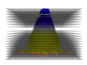
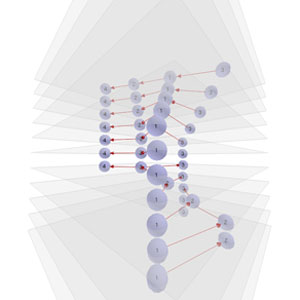
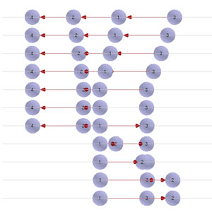
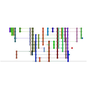
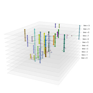
When a graph changes over a period of time (at discrete time steps), the entire process can be displayed simultaneously by using one layer for each time step and assigning the graph at the current time to that layer. Below are two examples:
Use case 2: Hierarchic structures

When a graph is hierarchical in nature, i.e. when multiple nodes can be successively grouped to form a more "high-level" representation of the graph, we can use one layer for each level inside the hierarchy. Below are two examples:
3. The goal of this project
The main goal of this project was to take an existing graph library capable of drawing 2D graphs and extend it with 2.5D functionality, i.e. to make possible the definition of 2.5D graphs, to define an interface for writing layout algorithms and to provide a mechanism for viewing and navigating 2.5D graphs.
Further, the following subgoals were defined:
- Integration into existing framework - This means using classes from the framework where possible and allowing 2D and 2.5D classes to coexist.
- Orthogonality - When defining new classes for the 2.5D case and similar functionality to the 2D case is implemented, use the same method names and paradigms.
- Expandability - Creating new layout algorithms and adding new information to entities of a graph should be easy.
- Visual appeal - The display of 2.5D graphs should produce nice pictures.
Finally, for testing and debugging purposes, an editor that allows creation and navigation of 2.5D graphs was considered useful.
4. Preparing to start
The library I chose for building the project upon was the yFiles library written in Java. Out of the box, it has some very advanced layout algorithms as you can check out yourself in the gallery section of the product page.
This choice also determined the language I used to implement the language: Java.
As far as displaying graphs in three dimensions goes, OpenGL seemed the natural choice. Luckily, a specification request is being worked on that exposes OpenGL functionality in the java language - it is termed JSR 231 - Java Binding for the OpenGL API. A reference implementation can be found at the JOGL home-page.
II. y25 - The Library
1. The y25 package - A bird's eye view
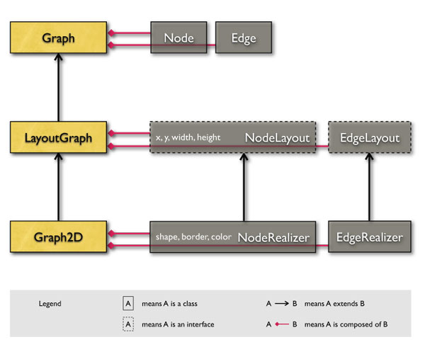
To understand the structure of the y25 package, one must first understand the basic structure of the yFiles package. The yFiles package is basically split up into three main packages: y.core , y.layout and y.view.
-
y.core holds the most important class of the entire yFiles package - the Graph. This class represents a purely abstract graph that is fully defined by G = (V,E).
-
y.layout builds upon y.core and adds layout information for nodes and edges through the interfaces NodeLayout and EdgeLayout. Layout information is composed of the position and extent of nodes and edges in 2D space. The central class that stores the graph together with the layouts is the LayoutGraph.
-
Finally,
y.view builds upon y.layout and defines the Graph2D as an extension to the LayeredGraph. The classes used to store layout information are NodeRealizer and EdgeRealizer. They additionally add visual information about nodes and edges such as their shape and their color and they are able to paint themselves into a Graph2DView that is also defined in this package. It can be used to display and navigate Graph2D instances.
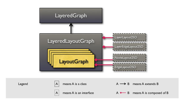
What follows is a compact visual overview of the yFiles class relationships:

Now to the 2.5D part: when extending the existing framework with 2.5D support, it seems very natural to mirror the existing hierarchy of packages and classes in the new framework. Therefore, the y25 package consists of the same main packages as the yFiles package: y25.core, y25.layout and y25.view.
-
y25.core hosts the most important class of the entire y25 package - the LayeredGraph. It is composed of layers and layer edges. Each layer is represented by a y.base.Graph instance, with in turn stores all the nodes and edges inside that layer. Layer edges are represented by LayerEdge instances. Up to this point, the information stored inside the layered graph is purely abstract, i.e. layers have no position or extent, neither do nodes, edges or layer edges.
-
y25.layout introduces the LayeredLayoutGraph which extends the LayoutGraph with layout information. Each layer is represented by a y.layout.LayoutGraph instance. Layout information for 2.5 dimensions is defined by the interfaces NodeLayout25D, EdgeLayout25D, LayerEdgeLayout25D and LayerLayout25D.
-
Finally,
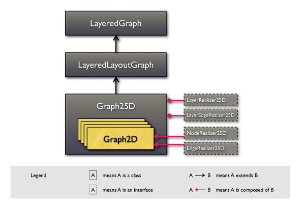
y25.view introduces the class Graph25D that represents each layer by an instance of y.view.Graph2D. 2.5D layout information is stored inside so called realizers that add 2.5D visual information to nodes, edges, layer edges and layers such as shape, color, etc..
These realizers can paint themselves into a Graph25DView that is also defined in this package. It can be used to display and navigate Graph25D instances.
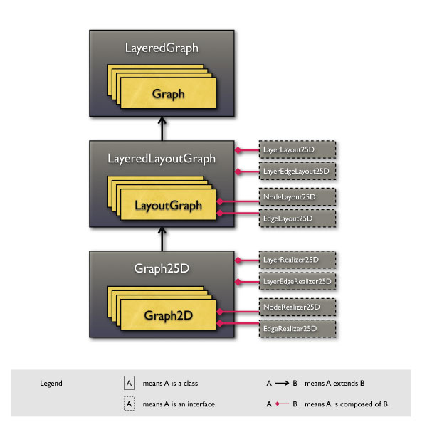
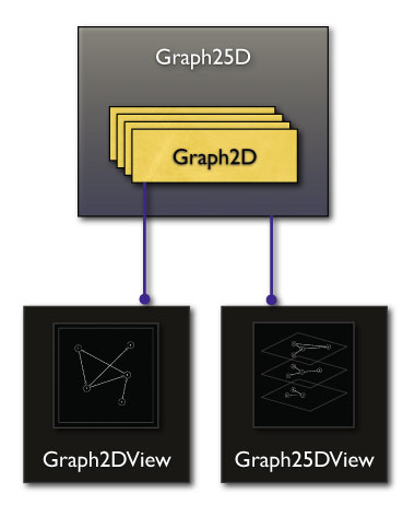
What follows is a compact visual overview of y25 and yFiles class relationships. (Layer edges, also stored inside the LayeredGraph, are omitted for clarity.)

There are a few points worth noting about this diagram:
-
First, it is important to understand that only the
LayeredGraph actually stores the Graphs in a list. All child-classes of LayeredGraph (LayeredLayoutGraph and Graph25D) use the same list, except that they store LayoutGraphs and Graph2Ds inside respectively.
-
Second, in order to provide compatibility with the yFiles package, the
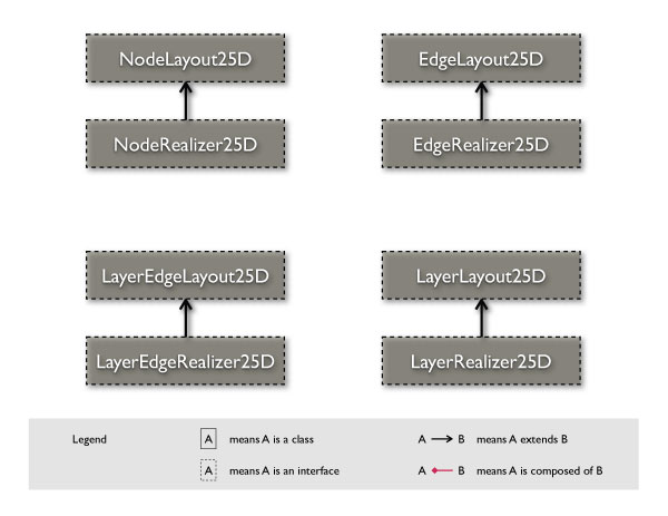
NodeLayout25D and EdgeLayout25D interfaces extend their counterparts form the yFiles package (NodeLayout and EdgeLayout).
-
As far as realizers are concerned, the situation is a bit more complicated - this is a topic discussed in the
y25.view section. One thing worth pointing out at this moment, however, is that in contrast to the yFiles package, realizers are not classes but interfaces.
In addition to the already mentioned core packages, the y25 library also includes the y25.graphics and the y25.io packages which are described in more detail in section 5 and 6 of this chapter.
2. y25.core - Working with abstract layered graphs
The y25.core package is composed of several classes, the LayeredGraph together with the LayerEdge being the most important of them.
a. LayeredGraph & LayerEdges
A layered graph is composed of graphs and layer edges. Each graph in turn is composed of nodes an edges. A schematic sketch illustrates this structure:

The graphs and layer edges are initially stored in the order of their creation. Of course, this order can be modified later by using methods of the LayeredGraph.
The mayor difference between layer edges and normal edges is that the latter are only allowed to have source and target nodes that lie inside the same layer whereas layer edges can start and end inside different layers. This is also the reason why layer edges are stored inside the layered graph and not inside the graphs that represent the layers.
As mentioned in the introduction, one use of a layered graph is to store multiple versions of a graph inside different layers. Another one is to store a graph at different time steps inside different layers. In these applications, nodes and edges inside different layers are logically the same (or at least related to one another). Therefore, the need arises to assign identifiers to nodes and edges inside different layers. The layered graph indeed has such a mechanism:
-
Every node inside a layered graph has its own "node ID". When a new node is created, it is automatically assigned an ID that has not been been used before. Valid node IDs are in the range from 1 to infinity. Of course, the automatically assigned node IDs can be changed later on by using
LayeredGraph methods.
-
Every edge inside a layered graph has its own "edge ID". Just like node IDs, valid edge IDs are in the range
[1,infinity), new and unique edge IDs are automatically created for each new edge and they can be changed later on by LayredGraph methods.
Another use of layered graphs mentioned in the introduction is to store multiple levels of a hierarchy inside different layers of the layered graph. Therefore, some nodes inside one layer may be the children of a node from another layer. Again, the need arises to be able to assign each node a parent node. The layered graph accomplishes this task by storing a "parent ID" for each node. By default, newly created nodes get a parent ID of 0, which means that they have no parent. Again, this parent ID can be changed by using LayeredGraph methods.
When creating a layered graph from scratch, the usual steps that have to be taken are the following:
-
Create a new instance of a layered graph.
-
Use that instance to create a graph each time a new layer is needed.
-
Specify the nodes and edges inside that layer.
-
Create layer edges between existing layers at any time.
Below is a code snippet that creates a simple layered graph with two layers, each with two nodes and one edge. Finally it creates two layer edges:
LayeredGraph layeredGraph = new LayeredGraph();

Graph firstGraph = layeredGraph.createGraph();
Node  node1 = firstGraph.createNode();
Node  node2 = firstGraph.createNode();
Edge  edge1 = firstGraph.createEdge(node1,node2);

Graph secondGraph = layeredGraph.createGraph();
Node  node3 = firstGraph.createNode();
Node  node4 = firstGraph.createNode();
Edge  edge2 = firstGraph.createEdge(node3,node4);

LayerEdge layerEdge1 = layeredGraph.createLayerEdge(node1, node4);
LayerEdge layerEdge1 = layeredGraph.createLayerEdge(node3, node1);
In the above example, if node1 and node3 are logically the same, the code below assigns them the same ID:
layeredGraph.setNodeID( node3, layeredGraph.getNodeID(node1) );
b. Utility classes
Cursors
When working with layered graphs, iteration over layers and layer edges is a common task. For this reason, iterator objects called cursors are defined for those entities. Note that iteration over nodes and edges of a single layer is the same as specified in the yFiles library. Here is an example for iteration:
// iterate over all graphs
for(GraphCursor gc = layeredGraph.graphs(); gc.ok(); gc.next()) {

	// get the current graph
	Graph graph = gc.graph();

	// iterate over all nodes of the current graph
	for(NodeCursor nc = graph.nodes(); nc.ok(); nc.next()) {
		Node node = nc.node();
		// do something with the current node
		...
	}

	// iterate over all edges of the current graph
	for(EdgeCursor ec = graph.edges(); ec.ok(); ec.next()) {
		Edge edge = ec.edge();
		// do something with the current edge
		...
	}
}

// iterate over all layer edges
for(LayerEdgeCursor lec = layeredGraph.layerEdges(); lec.ok(); lec.next()) {
	LayerEdge layerEdge = lec.layerEdge();
	// do something with the current layer edge
	...
}
Maps
When the need arises to associate application specific data to nodes, edges, layer edges or layers, instead of subclassing these entities another mechanism is provided: Maps. They can be created by a layered graph instance and can be used to store data for all nodes, edges, layer edges and layers inside that layered graph.
GraphTools
GraphTools is a collection of methods for duplicating graphs from the yFiles package. In addition to the graph copying process already provided by yFiles, these methods allow the user to specify which DataProviders should be copied as well.
c. Connections to the yFiles library
As mentioned before, the LayeredGraph uses instances of type Graph to represent layers. Since an automatic ID assignment process is responsible for creating new IDs for each newly created node or edge, it is recommended to create the graphs by using a LayeredGraph instance. However, if existing code written for the yFiles library wants to use the y25 package, it is possible to import graphs into a layered graph object by using the importGraph method. The standard behavior of this method is to assign new IDs to all imported nodes and edges just as if they were created at that moment. There is a way, however, to specify node, edge and parent IDs for the graph before importing it. See the API documentation for details on this subject.
There is another issue concerning the NodeMap and EdgeMap interfaces defined by the yFiles library. The documentation for these interfaces says that one map can only be used for nodes (or edges) that belong to the same Graph. This is a restriction that does not work well with the y25 package, where multiple graphs are used to build the layered graph. Users of the package might want to use a single map to assign values to nodes (or edges) that reside in different layers. This is why the y25.core package defines its own NodeMap and EdgeMap interfaces.
3. y25.layout - Bringing layout to layered graphs
a. What is layout information?
The LayeredLayoutGraph is the central class of this package. As described in the y25 overview section, it is responsible for storing the layouts of nodes, edges, layer edges and layers. For this task, the interfaces NodeLayout25D, EdgeLayout25D, LayerEdgeLayout25D and LayerLayout25D are used.
While layer and layer edge layouts are stored directly inside the LayeredLayoutGraph, node and edge layouts are stored inside each layer that is represented by an instance of a LayoutGraph. Below is a schematic sketch of this relationship:

But what is the layout information that needs to be stored composed of? The answer to this question is very important, since it mirrors the constraints that we set out to use for the display of graphs in three-dimensional space. Understanding these constraints that lead to a 2.5-dimensional graph structure is the key to understanding the y25.layout and y25.view packages. For this reason, all assumptions and constraints made about the arrangement of a graph's entities in three-dimensional space are listed below:
-
All objects live in a 3D world with a left handed coordinate system. Note that the choice of a left-handed over a right-handed coordinate system is somewhat arbitrary, but it makes sense when one of the goals of this project is very good integration with the yFiles library: a left-handed coordinate system allows to interpret the x- and y-coordinates of nodes and edges on left/right and upper/lower axes in both 2D and 3D space, while adding the z-coordinate can be interpreted as an elevation from the ground level where a positive z-coordinate means positive elevation.
-
Individual layers of a layered graph lie in planes that are parallel to the x/y plane. Therefore, each layer has an elevation that is represented by its z-coordinate. Layers are usually thought of as having no extent in the z-direction, i.e. they are a true 2D subspace of the 3D space they reside in. A layer's extent inside this 2D subspace can be described by an axis-aligned bounding box.
-
Nodes and edges inside a layered graph belong to a specific layer. This, together with their x- and y-coordinates completely specifies their 3D position, since the z-coordinate can be inferred from the layer they reside in. Therefore, storing the z-coordinate for nodes and edges would be redundant. Unlike they layers they reside in, however, nodes and edges can have an extent in the z-direction, so additionally to the node's width and height, its depth is also stored.
-
Layer edges have to start and end at a node. Therefore, the 3D positions of their endpoints can be inferred from their source and target nodes respectively. However, layer edges are allowed to have an arbitrary number of bend points that can be freely positioned inside 3D space. So in a sense, layer edges are the only "true" 3D objects of a layered graph.
While the above list gives an informal overview of what layout information consists of, the API specification of the aforementioned layout interfaces lists exactly how this translates to values that have to be stored (z-coordinates, the depth of nodes, bounding boxes, etc.).
It is important to note that the LayeredLayoutGraph is only an abstract class and therefore, it can't be instantiated (just as the LayoutGraph of the yFiles library). The main purpose of this class, then, is to define a minimal set of layout information that can be used for automatic layout algorithms. These algorithms are implemented in so called Layouter25D.
b. Layouter25D
Layout algorithms for graphs in 2.5 dimensions can be arbitrarily complex and they may differ a lot from one another. So only the most common ground of all these layout algorithms is captured inside the Layouter25D interface:
-
First, a
Layouter25D has to be able to answer the question of whether or not it is able to layout a given layered graph. This is done by implementing the canLayout(LayeredLayoutGraph) method.
-
Second, once the previous question has been answered with 'yes', the
Layouter25D has to be able to actually perform the layout process on the same layered graph. This is done by implementing the doLayout(LayeredLayoutGraph) method.
When writing a very complex layouter, it may be better to split it up into multiple distinct layout stages and to form a chain where one stage is executed after the other. This can be accomplished by the CompositeLayouter25D and LayoutStage25D interfaces defined in this package.
c. Connections to the yFiles library
There are many more layout algorithms for 2D graphs than for 2.5D graphs. Also, the yFiles library comes fully loaded with very advanced ready-to-use layout algorithms. For this reason, this package provides two mechanisms for applying those 2D layouts to 2.5D graphs:
-
The first possibility is to just perform a 2D layout process on each layer individually. While not very sophisticated, this approach might be useful in some situations. The
Layouter25DAdapter class is the way to go here.
-
The second possibility is to first "collapse" all layers of the layered graph into a single one, perform a 2D layout on the collapsed graph and then apply the calculated positions of nodes and edges to the original nodes and edges inside the different layers. The
FlatLayouter can be used to perform exactly these steps, where both the collapsing/uncollapsing and the 2D layout step can be specified by the user. A default collapsing/uncollapsing step based on the IDs of nodes and edges is also provided.
d. Example for writing a layouter
For an example of how to write a very simple layouter, see "Appendix A - The Centralizer Layouter" of this document.
4. y25.view - Displaying layered graphs
a. Graph25D
Simply put, the Graph25D is just an extension of the abstract LayeredLayoutGraph class that implements all the abstract methods defined there. Layout information for nodes, edges, layer edges and layers is stored inside so called "realizers", each extending the corresponding "layout" interfaces defined in the y25.layout package. In analogy to the LayeredLayoutGraph, realizers for layer edges and layers are stored directly inside the Graph25D, whereas realizers for nodes and edges are stored in each layer individually. For this to be possible, each layer is represented as a Graph2D:

Whenever a new entity (node, edge, layer edge, layer) is created, it automatically receives a default realizer. Each entity has its own default realizer that is stored inside the Graph25D.
Finally, a Graph25D can be displayed inside a Graph25DView - a class that is described later on.
b. Realizer25D
Realizer25Ds extend the Layout25D interfaces defined in the y25.layout package:

They add two important capabilities to the Layout25D interfaces:
-
Visual information such as the color or the shape of an object is stored.
-
They can paint themselves into a
Graph25DView by using OpenGL commands.
When actually writing a realizer for a layer edge or a layer, the only thing needed to make sure it works with the y25.view package is to implement the corresponding Realizer25D interface.
Writing realizers for nodes and edges is somewhat more complicated. The interfaces NodeRealizer25D and EdgeRealizer25D are not meant to be ever "used alone", but instead always together with their yFiles counterparts: NodeRealizer and EdgeRealizer. While the yFiles realizers are abstract classes, the y25 realizers are interfaces, so when creating a realizer for a node or an edge, one has to extend the Realizer class and implement the Realizer25D interface:

The reason why this is necessary is that node and edge realizers - in contrast to layer edge and layer realizers - have to be able to paint themselves into both a Graph2DView defined in the y.view package and into a Graph25DView defined in this package.
There would have been one alternative to this approach: the Realizer25D could have been made abstract classes that extend the Realizer defined in the yFiles library and extend the Layout25D interfaces from the y25 library. In this case, however, it would have been impossible to use existing realizers such as the ShapeNodeRealizer or the PlolyLineEdgeRealizer (due to Java's lack of multiple inheritance). Instead, all that existing functionality would have had to be programmed from scratch.
c. Graph25DView
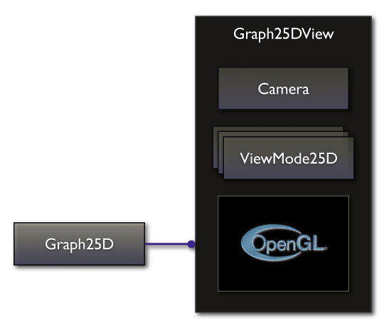
The Graph25DView can be used to display and navigate one instance of Graph25D. The paradigm of the display process is that the viewer looks through a virtual camera into the 3D world the layered graph lives in. When navigating through the graph (by means of a ViewMode25D that is explained later), various camera parameters are changed that affect the display process: the camera's view target, the view distance, the camera rotation, the "perspectiveness" of the camera (anything between orthogonal or overly perspective), etc.. For the actual display process, an OpenGL context is needed that is automatically created by the Graph25DView.
Below is a schematic view of the Graph25DView with its internal camera, its view modes and its OpenGL context. Additionally, the Graph25D associated with the Graph25DView is also shown with a blue link:

The display process performs the following steps:
-
Each realizer inside the associated
Graph25D is visited in turn.
-
The current realizer is asked to draw itself into the
Graph25DView by calling its paintGL() method and passing it the current camera parameters and the OpenGL context. Some realizers use the camera parameters to determine how to draw themselves, e.g. a node would draw its label in such a way that it always faces the viewer.
Finally, a Graph25DView can also be used to take a screenshot of the currently displayed graph and save it into a file.
d. ViewMode25D
View modes can be used to allow a user to "control" a Graph25DView through mouse inputs. "Control" here is meant in a very broad sense - in response to user actions, the view mode can change camera parameters, add nodes, edges, layer edges or layers to the currently associated Graph25D, etc..
A Graph25DView can hold any number of associated view modes. They need to be activated in order to receive user input events.
e. Connections to the yFiles library
The same that was true for the Graphs inside a LayeredGraph is true here as well: every newly created node or edge inside a layer that is represented by a Graph2D receives a new and unique ID by the automatic ID assignment process. Therefore, it is recommended to use the Graph25D instance to create the Graph2Ds that represent its layers. However, if code for the yFiles library exists that produces a Graph2D that needs to be included in a layer of a Graph25D, the importGraph() method has to be used.
Further, since all node and edge realizers stored inside the individual layers of a Graph25D have to extend the Realizer class and implement the Realizer25D interface, it is safe to use one layer of a Graph25D whenever a Graph2D is needed in the yFiles library. This is especially true for the Graph2DView. It is even possible to display the entire Graph25D in a Graph25DView and one layer of that Graph25D inside a Graph2DView at the same time! This setup is shown in the scheme below:

f. Example: Getting started with Graph25Ds
The code below sets up a small working environment that can be used to test y25.view functionality.
// First, we create a Graph25D
Graph25D graph25D = new Graph25D();

// Then, we may want to change some of its default realizers
ShapeNodeRealizer25D snr = new ShapeNodeRealizer25D();
snr.setShapeType(ShapeNodeRealizer.RECT);
snr.setHeight(30);
snr.setWidth(30);
snr.setDepth(10);
graph25D.setDefaultNodeRealizer25D(snr);

PolyLineEdgeRealizer25D er = new PolyLineEdgeRealizer25D();
er.setArrow(Arrow.STANDARD);
er.setDisplayMode(PolyLineEdgeRealizer25D.MODE_2D);
er.setLineColor(new Color(200,0,0));
graph25D.setDefaultEdgeRealizer25D(er);

TransparentLayerRealizer25D tlr = new TransparentLayerRealizer25D();
tlr.setRelativeBoundingBox(
    new BoundingBox(new Point3D(-200,-200,0), new Point3D(200,200,0) ) );
tlr.setOpacity(0.4f);
tlr.setRGB(250,250,250);
tlr.setZ(0);
graph25D.setDefaultLayerRealizer25D(tlr);

// Now, we create the Graph25DView and set some viewing parameters
Graph25DView view25D = new Graph25DView();
view25D.getCamera().setRotation(-90,0,0);
view25D.getCamera().setPerspective(30);

// To be able to interact with the Graph25DView, we create a ViewMode25D
ViewMode25D  navigationMode = new NavigationMode25D();
view25D.addViewMode25D(navigationMode);

// Finally, we associate the previously created Graph25D with the view
view25D.setGraph25D(graph25D);

// We are all done! Now the work on the Graph25D can begin:
// ... create new layers, node, edges, layer edges ...
// ... apply some layouter to the created graph25d ...
// ... etc ...
5. Utility classes
a. y25.io - Reading and writing Graph25Ds
In order to be able to save and load Graph25Ds, this package introduces the GMLIOHandler25D. This class can read and write 2.5D graphs in the GML format from and to files on the disk. At this moment, extending the IO mechanism is only supported by directly changing the GMLIOHandler25D code. Instead of doing this, however, I recommend writing a new IOHandler that stores graphs in the GraphML format (as opposed to the GML format), since it is based on XML and more superior.
b. y25.graphics - Linear algebra and OpenGL tools
When doing calculations in three-dimensional space, they are much easier to comprehend when using linear algebra concepts such as points, vectors, linear and affine transformations (represented as matrices) to express them. The following classes are therefore defined in this package:
-
Point3D - a point in three-dimensional space with a x-, y- and z-coordinate.
-
Vector3D - a direction in three-dimensional space with a x-, y- and z-component. The difference of two points results in a vector.
-
Transform - a transform that can be either linear, affine or projective (each successive type includes the ones before, e.g. an affine transform is also linear). At this moment, except for the matrices used inside the Camera to project points, only affine transforms are used in the y25 library. Internally, these transforms are stored as 4x4 matrices. Transforms can be applied either to other transforms, to points or to vectors. When applied to other transforms, a simple multiplication of two matrices is performed. When applied to points, the point is extended with a fourth coordinate - the homogeneous coordinate - of 1. A vector, on the other hand is extended with a homogeneous coordinate of 0. After that, applying the transform is simply a matter of multiplying the matrix with the extended vector. Even though this might be confusing at first, in our case it really only means that points are transformed by the full affine transform and vectors are only transformed by the linear part of the transform. To give a very simple example, if a transform performs both a translation and a rotation, then the point will be rotated and translated, whereas the vector will only be rotated.
Building on these fundamental concepts, the y25.graphics package further defines:
-
BoundingBox - an axis aligned bounding box that is specified by a minimum point and a maximum point.
-
Camera - a virtual camera that is used inside
Graph25DView to display the 3D world. The camera has several parameters that can be changed, such as its target view point, its rotation, its perspectiveness, etc.
Finally, there is another class defined in this package - Graphics3D - that can be used to draw geometric primitives such as cones and cylinders into an OpenGL canvas. It is mainly used by realizers, for instance to draw edges, arrow heads, etc.

